AIT614

Authors:

Neethu Battula, Sagar Goswami, Suchada Hapikul, Ewin Hong, Cross Zeigler

Abstract

New York City (NYC) is notorious for having heavy traffic at nearly all times of day, heavily impeding motor traffic in the city even at the best of times. It often leads to congestion that can delay travel and cause serious issues ranging from inflated costs of living to high gasoline prices. Therefore, it is very important for any changes in infrastructure to lead to more pedestrian-friendly roads and help people access public transportation easier, leading to less cars on the road over time. This project aims to study one or more datasets of traffic patterns of NYC and to create a model that predicts when traffic occurs the most hourly, daily, weekly, monthly, and annually. It will study this phenomenon by utilizing datasets from NYC open data to analyze traffic in the city, discovering commute patterns in transportation to resolve congestion among other traffic issues within NYC. Various analytical methods like K-Means Clustering, Time-Series Analysis, Multivariate Regression Models, and Decision Trees were considered to explore the data, and generate crucial insights that might fulfill the aforementioned goals. When performing the K-Means Clustering, it was observed that some of the sensors/link points behaved similarly in terms of daily average traffic speed. Two such clustering models were created that individually examined the average traffic speed, as well as the delta values for change in the average traffic speeds. On the other hand, the time-series analysis rendered different kinds of insights which focused on the variation/patterns in the average traffic speed grouped by hours of the day, days of the week, and months of the year. The data for 2018, 2019, and 2021 behaved very similarly, and mostly overlapped with each other when plotted on graphs for the Time-Series Exploration. The 2020 data showed similar traits, except it exhibited slightly higher traffic speeds compared to other years.

Introduction

New York City (NYC) is notorious for having heavy traffic at nearly all times of day, heavily impeding motor traffic in the city even at the best of times. This often leads to congestion which impacts travel and causes delays, wastes gas, and can leave people feeling dissatisfied with personal and public transportation. A prominent question for NYC, then, is how to improve the traffic infrastructure within NYC, leading to changes and improvements in transportation, pollution levels, and more. The main goal of this project was to study the datasets of traffic patterns of NYC and to create a model that predicted when traffic occurs the most hourly, daily, weekly, monthly, and annually. The thought was that this could help to consolidate which times of the year are “problem” times and allow people to adjust their commute accordingly before major infrastructure changes are made. Another thought that the researchers had for this project is that doing may even help change traffic patterns based on people’s ideal personal schedule, allowing someone to leave right on time to make traffic as smooth as possible for them and others. It became more important than ever this year to conserve gas not just for the environment but for personal use too as the cost of living, including gasoline prices, rises. The main motivation for completing these goals is to give insights into the NYC traffic system to give suggestions to improve it. Improving everyone’s personal schedule is a small stepping stone to accomplish this goal, but that is useless and a short-term solution without improving the actual infrastructure of NYC. These changes could lead to more pedestrian-friendly roads and easier access to public transport, reducing the number of cars on the road over time. To accomplish this, the experimenters attempted to look over the specific areas of congestion along with the times there is little to high congestion. The thought was that by looking over the areas of high congestion they could find a way to reroute traffic to make those areas less busy. Looking over times of congestion helped to reveal how traffic changed over time and allowed the researchers to theorize why these changes occurred due to holidays, construction, or other events. The end goal was to advocate for public policy to refine infrastructure. Several audiences could benefit from this analysis. The primary audiences are the stakeholders in the urban transportation industry and transportation agencies. For both, if people have an easier time moving around, they may be more inclined to utilize public transportation, which could drive revenue up. The latter in particular may like this, as they have a lot more to gain directly from people using their services more. Two other audiences are emergency services and NYC residents. Ambulances and firetrucks need to get to their destinations quickly to maximize the amount of lives they save and the chances of saving said lives. With NYC as it is, even if people try to maneuver out of their way, they still have to deal with traffic regularly that could impede their progress. NYC residents would not just appreciate this ease of access emergency services have to save their lives, but also in day-to-day life. Someone may struggle to get to work on time or meet up with friends if they constantly have to battle heavy traffic. Changing infrastructure could help improve satisfaction with living in NYC, improve work ethic and punctuality, and lead to increased happiness with one’s social life by ease of access alone. Attempting to improve NYC’s traffic situation is not new. People have studied this issue extensively in hopes of understanding why traffic is so bad in the city and how to improve it over time. Nibareke and Laassiri (2020) used various machine learning models to model traffic flow over time to predict traffic effectively. While they specifically dealt with air traffic their model allowed people to see how accurately one could predict delays and traffic in transportation with the correct model. Vasudevan (2016) presented a technical approach that combined Apache Spark’s open-source data analytics and machine learning techniques to predict traffic flow patterns using simulated connected vehicle messages. The study reported that connected vehicle data can be processed rapidly using Big Data analytics to generate precise predictions of traffic flow regimes. Other researchers reviewed had similar results.

Goals

The primary goal of this project is to create a machine learning model to predict the traffic within NYC based on the NYC traffic statistics collected from the New York City Department of Transportation website. Looking over times and the specific areas of congestion can assist audiences to know how traffic changed over time. This project aims to provide valuable insights into the NYC traffic system to improve transportation infrastructure for increased satisfaction, safety and decreased travel time. Providing audiences with the times and areas with the greatest amount of congestion may allow people to leave their locations at the optimal times to make traffic as smooth as possible for them. Thus, they can improve their own commuting schedule and potentially increase their own safety. Improving personal schedules is a small stepping stone to accomplish reforming traffic infrastructure within NYC for the long term. The long term goal of this project is to improve the infrastructure of NYC. While the short-term goal can help individuals and perhaps even large collectives of people, it may only support so many people for so long. During the short-term goal’s tenure, NYC’s departments for transportation and infrastructure could make plans to fix and reform the public transportation and infrastructure of the city. That way, commuting schedules amongst other problems would not fall completely on individuals and instead cater to them for consistently reliable transportation. This project intends to improve commuting schedules in the short-term by improving personal schedules, but the ultimate long-term goal is to affect policy for the improvement of NYC’s infrastructure.

Requirements & Methodology

The project has several functional requirements. The requirements for analysis include several tools from programming languages to visualization tools. This project uses R Studio for extracting, processing, cleaning, and exporting data. R is easy to use and provides a tool with a good amount of complexity combined with a low entry bar to help with initial analysis. Thus, R was utilized for both data exploration and deeper data analysis as well due to it affording users the proper tools to do so. Moreover, R also provides clear graphs and outputs that help to create a data story for projects. In addition to this, the earth library was used to attempt to run a more complex MARS analysis on the data. The second main analysis tool used is Python. The project used Python for data cleaning and analysis with specific libraries such as Pandas. Python combines many of R’s strengths from good visualizations for data stories, a great breadth of data analysis tools, and a low bar for entry, especially if one is familiar with Java or C. The language has many libraries that assist with these tasks, including the aforementioned Pandas which helps with extracting, processing, and cleaning data. Alongside R, Python was used to store the data initially in order to do rudimentary exploration so that one could familiarize themself with what the data may mean. Python’s libraries such as prophet gave access to more complex analysis such as the time series analysis, pushing the project further along. The main platforms used for this project were Databricks, Apache Spark, GitHub and Microsoft Teams. Databricks provided many of the languages and other tools necessary to perform the analysis, and served as a better storage tool for the data in the long-term relative to other platforms. Databricks DBFS specifically was used as a NoSQL database to handle the large volume of data from the original dataset. Databricks also served as a decent collaboration tool for multiple people to modify the code together in real time, circumventing any issues of having to meet in-person for the project. Apache Spark and its corresponding libraries (i.e. Spark MLlib) were used for most of the more complex data analysis, such as principal component analysis (PCA) and k-means clustering. Spark also provided access to SQL and R on Databricks for visualization and the use of more complex libraries relative to other platforms. These languages gave quick insights into the data with simple queries that could be visualized easily. The primary platform for communication was Microsoft Teams. Teams worked as a central hub for most meetings and information exchange. Even if a person were to miss a meeting, it was easy and quick to update them on the current status of the project by posting a summary of what was accomplished on Teams right after the meeting. Teams also held a number of the files for the project, including coding files, documentation on the code, and reports on the project. This way, people had unhindered access to the files they may need for analysis or directions. Google Docs was used in tandem with Teams, as it provided an easy way to share and create files for reports as well. In addition to that, Docs provided a running “meeting” file that recorded what went on in each meeting. A Google Drive was eventually established that held every report necessary for the project and was accessible to every group member. GitHub was the last main collaborative tool, and was used alongside Databricks for ease of code access and editing. Everyone had access to the original repository that hosted the code and could push for changes from a cloned repository. GitHub served as an excellent platform to track the coding progress of the project, and could be used to control which version of the project came to fruition better than Databricks could in many cases. It also served as the home of the documentation on how to run the project.

The Datasets

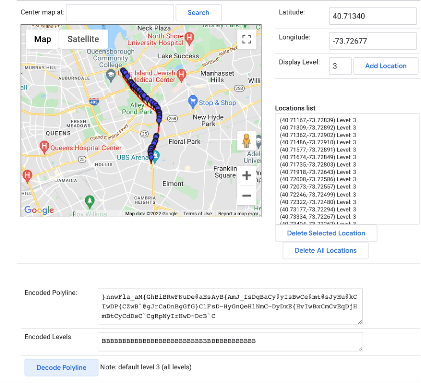
The dataset is collected from the New York City real time traffic speed found at: https://data.cityofnewyork.us/Transportation/DOT-Traffic-Speeds-NBE/i4gi-tjb9 (The NYC Department of Transportation website). The dataset is gathered in. As of March 9th, 2022, the dataset has 58.8 million records starting on April 17, 2017. The dataset is continuously updated with real time data being provided by the traffic sensors. There are 13 features listed found as table 1 in the Appendix. With these 13 features, 8 features are useful for the research. These eight features are id, speed, travel time, data as of, link points, owner, borough, and link name.
Speed in this dataset is the average speed between all of the link points. Travel time is time spent through the link points. The link points are a group of latitude and longitude points. The link point can be used to calculate the distance of the starting and ending points of a single link. Additionally, distance could be calculated by using speed and travel time as means of validating the calculated distance by link points. These link points can be evaluated over time and their evolution. Then with the link points, the Boroughs can be added for grouping for additional analysis. Each link point has at least 2 points and could go to 10 points. Due to the dataset, there is some evidence there might be more than 10, but are cut off due to the original dataset’s database type constraint of 256 characters.

Table 1

Name of Feature	Description	Data Type
ID	Unique Identifier for Sensor within dataset	Integer
Speed	Average Speed traveled between the link points origin and destination	Double
TravelTime	Time Travel in seconds	Integer
Status	Artifact (not useful)	Integer
Data_As_Of	Date and Time of Day for Sensor Data	Datetime
Link_Id	TRANSCOM Link ID	Integer
Link_Points	Group of Latitude and Longitude points of Sensor data	List of 2 double (latitude and longitude) points
Encoded_Poly_Line	Link_Point representation of Google compatible poly line	String
ENCODED_POLY_LINE_LVLS	Encoded representation of Poly Level	String
Owner	Owner of Sensor	String
TRANSCOM_ID	Artifact (not useful)	String
BOROUGH	Name of Borough Sensor exists	String
Link_Name	Description of Sensor location	String

The System

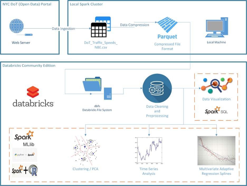
In the finalized project, the systems framework consisted of several modules/tools used to complete the project. The data was first gathered from the source and turned into a CSV file around 25 GB in size. To make the data easier to process, this CSV file was converted into parquet files that anyone experimenting with the project could feed into the algorithms to run to avoid storage and performance problems the CSV may have provided. Most of this was done on a local machine due to the power said machines provided relative to other platforms. After this occurred, the data was stored on the Databricks DBFS. Here, the data was cleaned and processed. Most of the code to clean the data was done in Python, with a focus on removing data that was extraneous and useless. To measure how useful the data was, the average speed was calculated (i.e. 34 mph), and no speed more than two standard deviations (15 mph for one standard deviation) going above this speed were kept. The range of kept speeds became 0 to 68. There was some debate on whether to keep all speeds that were 0 mph based on this criteria as well, but ultimately nothing was found using a similar criteria to eliminate data points with a speed of 0 specifically. After this, the link IDs were grouped together and the number of times each ID appeared was counted. If any IDS had less than 45,000 records, they were removed due to not contributing too much to the analysis and providing little to no interesting insights. Additionally, the year 2017 was omitted because the data was not consistently stored for that year, leaving many open gaps. The first major analysis utilized was K-means clustering to determine which link IDs had similar speeds and potentially why. PySpark was used for this, and the Spark MLlib library was utilized specifically for clustering. The 24 features from the cleaned dataset were fed to the k-means and PCA algorithms to determine the potential number of clusters. After this, a clustering evaluation was performed with Spark MLlib to determine the optimal number of clusters from 2 to 10 clusters, with the algorithm providing an answer of 3 clusters. After this, PCA was performed on the standardized features of the data. The three clusters were mainly divided by their speeds and the ranges of said speeds and locations, and each cluster’s link IDs were graphed on a box and whisker chart to determine their ranges of speed. The cluster having the lowest speeds typically were located near bridges and had the lowest range of values for each link ID while the cluster with the highest speeds had the largest range of values for each link ID. The cluster with lowest speeds typically had average speeds lower than 30 mph while the cluster with the highest speeds had average speeds well above 30 mph. The next major analysis performed was a time series analysis to determine traffic trends for the past several years and to predict trends for the next two (up until 2024). To do this, Facebook’s Prophet library was installed and fed two values: the datetime and the speed. While link IDs were grouped together in this instance, most of the visualizations featured were for an overall, general trend on an hourly to yearly basis. The FBProphet method then used the speeds from 2018 to March of 2022 to find a trend line for viewers to follow, establishing how speed changed over time and even returning delta values for this change in speed over specific durations. Afterwards, the algorithm predicted what the speed trend would be for the rest of 2022 to 2024 based on the trend established from 2018 to 2022. This data provided an approximate view of congestion, and when grouped by link IDs, could give an idea of which areas were most congested (low speeds) and least congested (high speeds) overall and at certain times of the year. SparkSQL was also used extensively for time series analysis and for initial analysis of the data. Additionally, the data was aggregated for every hour to calculate the average speed for all of the records and link IDs. There was an attempt to perform two other types of analysis, those being decision trees and Multivariate Adaptive Regression Spline (MARS). MARS was performed in R code while decision trees were performed in PySpark, but several issues prevented any fruitful analysis from either. Even on a sample of the data (100,000 records vs. tens of millions of records), the algorithm took too much time, sometimes hours even. One reason was that fitting splines on top of linear functions increased the time of performance. Another issue for MARS in particular was a lack of libraries to properly visualize the data, as modern libraries did not have the capabilities most of the time and older libraries often lacked this functionality altogether. Finally, the time series analysis provided better results for a comparatively shorter period of time and lower resources overall, pushing time series analysis as the better tool. Beyond these algorithms, very few were used for data analysis For hardware, there was a mixture of computers and OSs running the algorithms. Several people utilized Macs with at least 8 GB of RAM, with one even having 64 GB of RAM. One user had a Windows machine that had 16 GB of RAM. Most of the OSs running on each machine were up to date as well to ensure quality performance and to be compatible with the most modern software available. For software, most versions of the programs used were the most current ones or near the most modern ones, with most users utilizing Python version 2.7 or above and R version 3.0 and above. Additionally, Databricks was used in performing exploratory tasks and executing computational heavy tasks like k-means and times series analysis. Each team member had their own Databricks community edition. A team based Databricks was established in both Amazon Web Services (AWS) and Google Cloud Platform (GCP) to collaborate together where the Databricks community edition could not provide this level of feature. In Databricks, various levels of clusters were used but common cluster configurations were one driver and one worker with 28 GB of RAM and four Core processors or 58 GB of RAM and 16 Core processors.

Experimental Results & Analysis

The project started with two techniques, those being K-means clustering and linear regression. The initial linear regression was found to be too simple for the project, so the aforementioned MARS analysis was employed in its place. Over time, several other techniques, including decision trees, time series analysis, and association rule mining were attempted as well. The final analysis and outcomes included the clustering and time series analysis, as the libraries needed to perform or optimize the other techniques were not available on the versions of the software utilized.

K-means

The clustering analysis attempted to group together the remaining link points based on their speed. Each link point had 24 features for average speed for an hour in the day. A clustering evaluation was performed to determine the optimal number of clusters for the data, and by measuring those speeds and how large or small they were relative to each other, three groups were established based on speed.

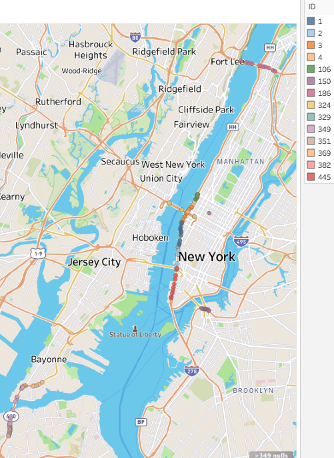
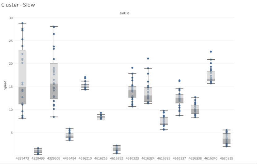
As observers can see above in the box-and-whisker plot, cluster 1 had 14 link points in it, making it the smallest cluster. Cluster 1 had the link points with the lowest speeds on average, typically speeds of 30 mph or below. These link points also usually had the least amount of range in their speed values relative to the other clusters’ link points, with a dozen having ranges of 10 or ;less and only two having a maximum range of 20. These link points were thought to be the ones located at the highest points of congestion, as car’s recorded as having lower speeds are usually either 1) in areas of high congestion or 2) have to be stopped due to a stop light or other obstruction. This is supported by the map seen above the plot, as most of these link points highlighted on the map are near the Manhattan borough or bridges and toll roads. Bridges can serve as a bottleneck for vehicles, as they are narrow passages that have few exits to remove excess traffic from quickly, leading to high amounts of congestion. Toll roads can serve a similar purpose, with the main difference being that cars must slow down for the toll to be paid, effectively creating traffic due to said slow down. The Manhattan borough contains many of the bridges in the NYC area, making it slow to enter and leave as a consequence.

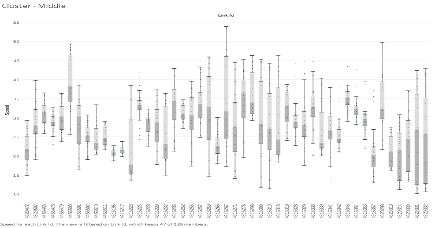
Cluster 2 is the “middle” cluster, containing the second highest number of link points and the “average” speeds. This cluster typically contained link points with speeds of between 20 mph and 50 mph, with there being a few link points with speeds ranging from 10 mph to 55 mph. Most of the link points relative to cluster 1 also had larger ranges of speeds, implying a higher variance in the amount of congestion this cluster had to the first one.

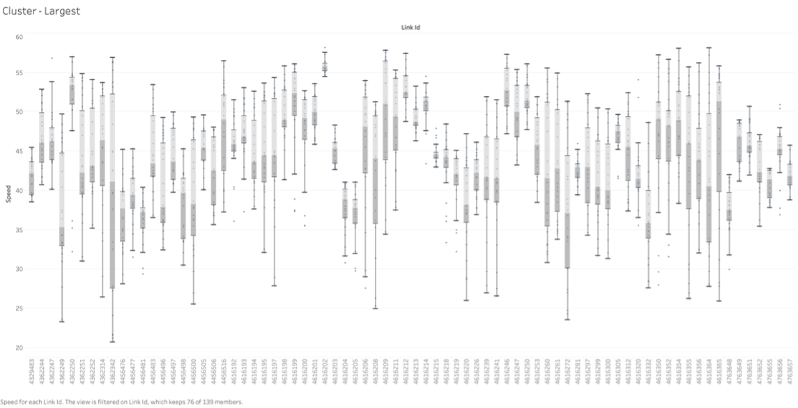
The third cluster, cluster 3, had the largest amount of link points and the link points with A) the highest speeds, reaching up to 60 mph, and B) the largest range in values for speeds per link point. The speeds for these link points were only as low as 20 mph if that. Like cluster 2, the high range of speeds per link point may be due to these link points having a larger range of landscapes, being a mixture of bridges, highways, streets, and more.

Time-Series Analysis

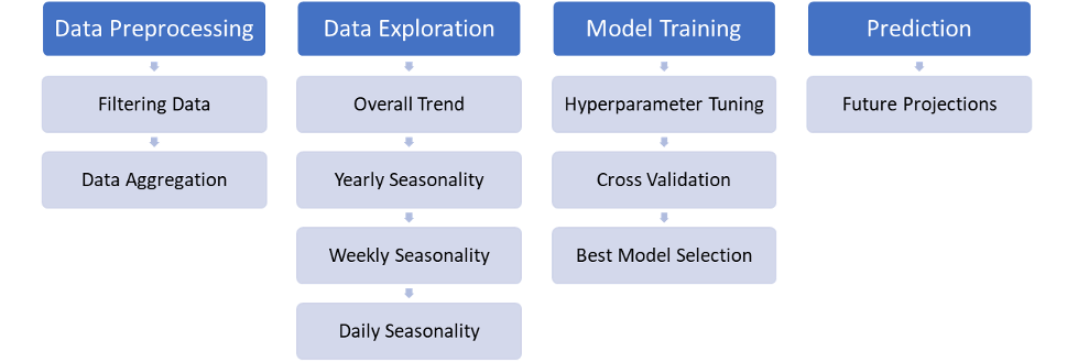
The time series analysis was carried out in following steps:

FBProphet allowed for the creation of a historical model of speed and was then used to create a predictive model for the overall trend of speed in NYC. The analysis also created a further breakdown of data by link points and for specific time periods from by the hour to annual speeds.

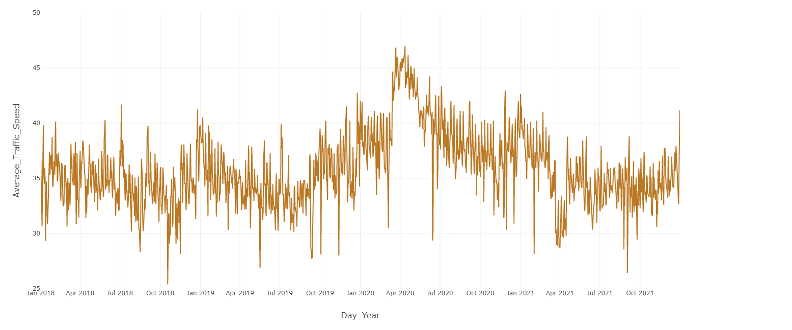
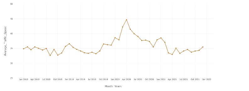
The overall trend of the data revealed the average speed stayed between 30 and 40 mph for most years, but towards April of 2020, the speed spiked to 45 mph. This was likely due to the COVID-19 pandemic leading to less cars everywhere as most people were ordered to stay home. This in turn led to less traffic and other obstructions, allowing drivers to navigate roads at higher speeds than usual.

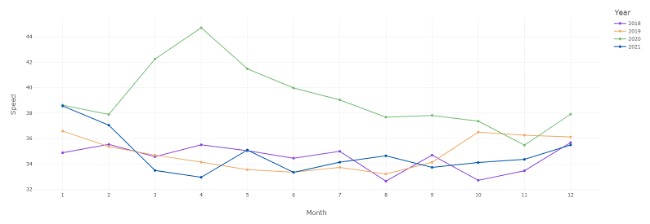
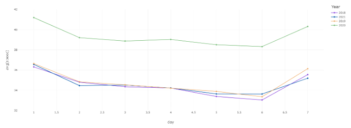
The yearly pattern featured above saw a similar pattern to the overall trend: most years had a speed between 32 to 40 mph, while the year 2020 had a notable increase in speed up to 45 mph. The first graph displaying the average speed in a year by month shows that the years 2018, 2019, and even 2021 follow this pattern, but 2020 saw a spike in speed around late March and early to mid April as the pandemic’s lockdowns occurred. Said lockdowns reduced traffic as mentioned before, allowing for higher travel speeds in automobiles for that period of time. As the year went on, the speed steadily dropped to the normal range of speed between 32 mph and 40mph as people began to return to their offices. There was a slight spike in speed in 2020 in November and December that may be explained by holiday travel: while less people traveled for the Thanksgiving and Christmas holidays, a notable number still did, and with less people on the road, those who did travel could travel at higher speeds. The speed eventually returned to pre-COVID levels in March of 2021 and stayed that way throughout the year, an indicator of people returning to some semblance of pre-COVID life, including driving patterns.

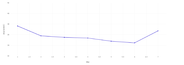
Weekly speed patterns saw most traffic occurring around Friday after a steady speed throughout the week. This was the case regardless of the year, although it should be noted that weekly speeds for 2020 were notably higher overall than for 2018, 2019, and 2021 as a result of the pandemic mentioned beforehand. The steady speeds, typically of 34 mph to 36 mph, from Monday to Thursday are likely due to this being the time of the regular work week, when most people are busy with navigating to and from work and not en masse for recreational activities. All years with the exception of 2021 to some degree saw a notable dip in speed around Friday and Saturday, going from a solid 34 mph or above to 32 mph. This is likely the consequence of the work week ending and many inhabitants utilizing transportation more than they would regularly for recreational and personal, non-work related needs. The speed began to rise on Sunday, likely when people weren’t doing as many recreational activities and work, leading to less people on the road. This afforded everyone who was driving on Sunday the ability to navigate the roads quicker with less obstructions.

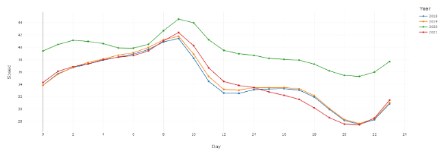
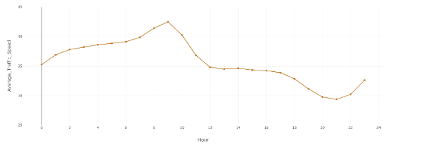
The next large patterns were daily speeds and the hours which saw the most congestion. Every year saw the speed begin to decrease around 8am from 42 mph to 36 mph from 12pm to 5pm. This could be explained by people beginning their commute between 8am and 9am, leading to higher volumes of traffic for the next several hours. The overall, slower speed that plateaued at 36 mph from 12pm to 5pm could be the result of everyone being at work and only leaving during that time for lunch. After 5pm, there was a sharp decrease in speed from 36 mph to below 30 mph around 8pm. The speed’s decrease at this time is likely due to everyone beginning to leave work, which may mix with the moderate amount of traffic that was seen in the plateau from 12pm to 5pm. This led to a higher amount of traffic than the earlier hours of the day due to the higher volume of cars around this time, explaining the sharp decrease in speed. This could be explained further by knowing where these cars were going the most often, such as to the aforementioned Manhattan borough which requires bridge access to reach leading to vastly lower-than-average speeds. The speed began to increase around 9pm from around 28 mph to around 42 mph. The speed then stopped increasing around 8am, when the work day began. This sharp increase in speed is probably the consequence of most people being at home during this time and resting during the night, leaving the people on night shifts as the primary demographic of drivers.

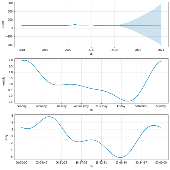
The final graph represents the best time-series model obtained performing hyperparameter tuning and cross-validation. Various hyperparameters were tested, and cross-validation was performed for every 180 day interval (over 4 years of data), which translates to an 8-Fold Cross Validation. It shows the future projection of how the speed may change on a yearly, weekly, and daily basis. The speed in the trend line for the year is mostly linear with a slight bump in 2020 due to the COVID-19 pandemic. If NYC’s physical and social architecture stays the same, the yearly speed will likely be the same as it has been in 2018, 2019, and 2021. The projected daily speed also matches up with the historical daily speed: high speeds on Sunday, a steady lower speed from Monday to Thursday, and a drop in speed on Friday and Saturday. Finally, the projected hourly mostly matches up with historical hourly speeds, with there being high speeds during the nightly hours after 9pm to early morning around 8am, then a progressive decline in speed up to between 5pm and 8pm.

The Summarized Project Timeline

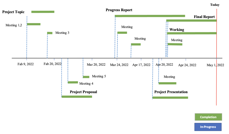
The project took place over the course of three months, starting in early February with the formation of the initial group up until the start of May with the final deliverable’s submission. As observers can see in the timeline above, every individual task is marked with a pin that has a tail with the assignment’s status: either being “in-progress” (blue) or “completed” (green). Additionally, there was a third category named “duration” colored gray, referring to tasks that hadn’t been started yet. Each pin’s tail extends for the rough duration of the project its respective task occurred under, e.g. the progress report was planned to start around March 24th, 2022, and was worked on up until its due date, April 24th, 2022. At the time of writing this, the final report and working system is being finalized, and should be complete by the due date, making them green upon turn in.

Conclusions

For overall conclusions, the project unveiled how speeds generally changed over time for a duration and typically where speeds were the slowest or highest. The cluster analysis revealed that 14 link points have a slower-than-average speed, usually below 30 mph, and most of these link points were concentrated around places where mobility was impeded such as bridges, toll roads, and places that had these structures in abundance such as the Manhattan borough. It may be favorable to find other ways to divert traffic to keep a high rate of traffic flow for increased travel speeds and lower travel times. Another conclusion was that the year 2020 saw a vast decrease in traffic due to the pandemic keeping most people inside, allowing people that did drive to do so faster with less obstructions and hazards. This may give insight into how NYC could schedule their workers’ deployment, minimizing the amount of people on the road at any time to keep a high traffic flow for convenience. The project gave the researchers an opportunity to work within many collaborative environments, some of them for the first time. The people working within said environments had to learn not only how to utilize the hard skills of file systems, coding, and organization, but the soft skills of collaboration, scheduling and dividing up responsibilities based on experience, skills, time, and other factors. Managing the schedule was a very important skill in particular to learn, as without the schedule, the project was delayed at times unexpectedly relative to overall deadlines and suffered from a lack of direction. Another lesson learned was how to identify the tools needed for the analysis for this project and interpreting traffic patterns with what few attributes there were in the initial dataset and analysis. This meant looking up complementary sources to the project to learn what levels of speed meant and if they matched up with other research or not.

Future Considerations

In the future, it may be optimal to use more datasets for better cross checking of the raw data and to utilize more attributes in the analysis such as travel time and the number of cars on the road. Other additional features could also include the number of lanes, foot traffic and how it impacts cars, and which way traffic flows (one-way, bidirectional, cardinal directions). A geospatial analysis could give better outcomes as well by determining the flow of traffic in areas and being used to recommend start and end destinations for drivers.

Works Cited

• Chen, H., Rakha, H. A., & Sadek, S. (2011). Real-time freeway traffic state prediction: A particle filter approach. 2011 14th International IEEE Conference on Intelligent Transportation Systems (ITSC). https://doi.org/10.1109/itsc.2011.6082873
• City of New York Department of Transportation. Retrieved on March 9, 2022 from: https://data.cityofnewyork.us/Transportation/DOT-Traffic-Speeds-NBE/i4gi-tjb9
• Das, A. (2021, February 10). K means clustering using pyspark on big data. Medium. Retrieved May 3, 2022, from https://towardsdatascience.com/k-means-clustering-using-pyspark-on-big-data-6214beacdc8b
• Diagnostics. Prophet. (2022, April 4). Retrieved May 3, 2022, from https://facebook.github.io/prophet/docs/diagnostics.html
• Dobilas, S. (2020, November 28). Mars: Multivariate adaptive regression splines - how to improve on linear regression? Medium. Retrieved May 3, 2022, from https://towardsdatascience.com/mars-multivariate-adaptive-regression-splines-how-to-improve-on-linear-regression-e1e7a63c5eae
• Elsyifa. (2019, February 24). Clustering-pyspark/clustering using pyspark_v2.ipynb at master · ELSYIFA/clustering-pyspark. GitHub. Retrieved May 3, 2022, from https://github.com/elsyifa/Clustering-Pyspark/blob/master/Clustering%20Using%20Pyspark_v2.ipynb
• Hofleitner, A., Herring, R., & Bayen, A. (2012). Arterial travel time forecast with streaming data: A hybrid approach of flow modeling and machine learning. Transportation Research Part B: Methodological, 46(9), 1097–1122. https://doi.org/10.1016/j.trb.2012.03.006
• Kulkarni, P. (2021, August 10). Tutorial : K-means clustering on Spark. Datasset to Mindset. Retrieved May 3, 2022, from https://www.data4v.com/tutorial-k-means-clustering-on-spark/
• Kong, F., Li, J., Jiang, B., Zhang, T., & Song, H. (2018). Big data‐driven machine learning‐enabled traffic flow prediction. Transactions on Emerging Telecommunications Technologies, 30(9). https://doi.org/10.1002/ett.3482
• Mourcos, A. (2019, June 6). Using PCA and K-means for Clustering. Using PCA and K-means for clustering. Retrieved May 3, 2022, from https://andrewmourcos.github.io/blog/2019/06/06/PCA.html?msclkid=658ba0e2bcea11ecbea027e6fdcfaf6c
• Nibareke, T., & Laassiri, J. (2020). Using Big Data-machine learning models for diabetes prediction and flight delays analytics. Journal of Big Data, 7(1). https://doi.org/10.1186/s40537-020-00355-0
• Obeidat, B., Smith, B., Heintz, B., & O’Malley, K. (2021, April 6). Fine-grained time series forecasting with Facebook Prophet updated for Apache Spark 3. Databricks. Retrieved May 3, 2022, from https://databricks.com/blog/2021/04/06/fine-grained-time-series-forecasting-at-scale-with-facebook-prophet-and-apache-spark-updated-for-spark-3.html
• Quick start. Prophet. (2022, April 4). Retrieved May 3, 2022, from https://facebook.github.io/prophet/docs/quick_start.html#python-api
• Vasudevan, M. (2016). Big data analytics: predicting traffic flow regimes from simulated connected vehicle messages using data analytics and machine learning. US Department of Transportation. Retrieved March 14, 2022, from https://rosap.ntl.bts.gov/view/dot/32616
• Yisheng, L., Duan, Y., Kang, W., Li, Z., & Wang, F. Y. (2014). Traffic Flow Prediction With Big Data: A Deep Learning Approach. IEEE Transactions on Intelligent Transportation Systems, 1–9. https://doi.org/10.1109/tits.2014.2345663